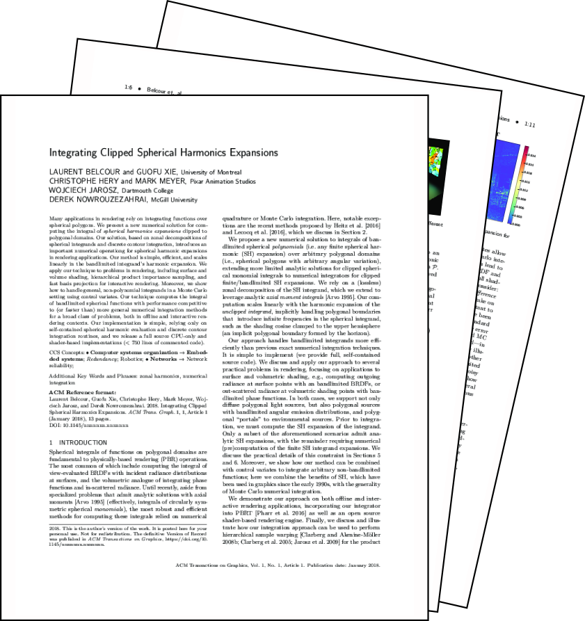
Integrating Clipped Spherical Harmonics

Laurent Belcour - Guofu Xie

University of Montreal

Christophe Hery - Mark Meyer

Pixar Animation Studio

Wojciech Jarosz

Dartmouth College

Derek Nowrouzezahrai

McGill University

Motivation

Spherical Integrals are common in rendering
- Shading on surfaces
- Shading in volumes
- Importance sampling
- ...

Analytical forms are not common

But are needed by real-time rendering

Motivation: BRDF Integration

(Quasi) Monte-Carlo
- Approximative (contains error)
- Large number of samples
Real-Time Rendering
- Sampling is out of the question
- Needs efficiency, allows approximate
Analytical solutions are welcome
- Must include the light (spherical domain)

BRDF

light

To further illustrate this point, let's take the example of direct lighting of an opaque surface. Say we want to compute the reflected radiance of the surface in the white pixel here illuminated by this area light.*click*

For the view vector of the pixel here in red, the bidirectional reflectance distribution function defines the function to integrate. And this integral is restricted to the spherical polygonal defined by the projection of the area light.*click*

In the offline community, the default is to rely on (quasi)-random integration using Monte-Carlo. There, we importance sample directions in the area light or with respect to the BRDF and compute the average. However, in the general case, this solution is an approximation as we will always obtain a noisy/incorrect estimate. It would require an infinite number of samples to get the true value. *click*

But if we look at real-time constraints, using many samples is out of the question given the rendering budget at hand. However, there it is often possible to trade correctness for efficiency and have approximate (yet non-random) answers. *click*

Thus, we seek for analytical solutions of spherical integrals.

A Few Existing Methods

Polygonal lights

[Arvo 1995] [Heitz et al. 2015]

Sphere lights

[Dupuy et al. 2017]

Linear lights

[Heitz et al. 2017]

But restricted to specific spherical functions

Our Solution

Integrate Spherical Harmonics expansions on spherical polygons
Efficient algorithm
- scales well with higher order SH
We incorporate such analytical solution
- for shading on surfaces
- for shading in volumes
"What about shadowing/bias ?"
- using control variates
- or a ratio estimator [Heitz et al. 2018]

So we looked at a broader set of spherical functions that are spherical harmonics. Spherical harmonics are a basis of function that are already used in many application where the spherical distribution to approximate has no specific shape. For example, it is common to use them to bake lightmaps for video games. In this talk, I will show how to integrate those functions over spherical polygons. *click*

We also managed to solve this problem in an efficient way that scales linearly with respect to the number of spherical harmonics coefficients. *click*

In our paper, we show how to incorporate those integrals for surface shading and volume shading. *click*

But we can also incorporate shadowing of the light source using control variate. We use it as well to reduce the approximation error made by the spherical approximation. Note that our solution works as well for the ratio estimator of Heitz and colleagues which is another form of control variate.

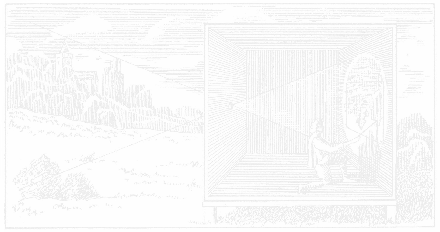
Inspiration: Axial Moments

Function of the dot product, $f(\omega) = \langle \omega \cdot \color{red}{\omega_i} \rangle^\color{green}{n}$
Recursive integration [Arvo 1995]
- Linear with respect to the power $\color{green}{n}$
- Each step integrate another power cosine

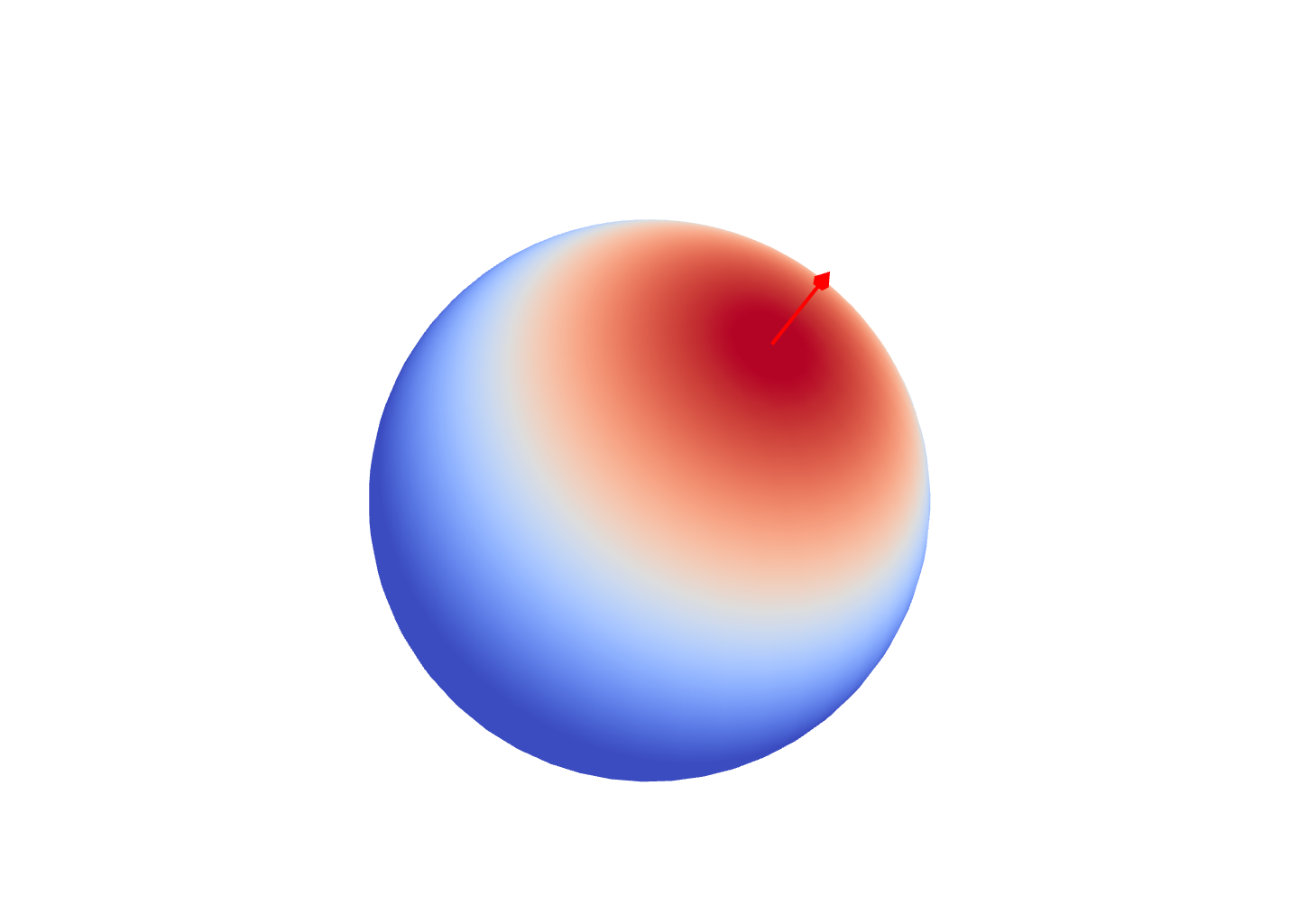
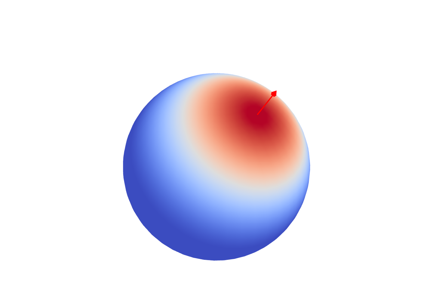
$\color{red}{\omega_i}$

$\langle \omega \cdot \color{red}{\omega_i} \rangle^\color{green}{3}$

$\langle \omega \cdot \color{red}{\omega_i} \rangle^\color{green}{5}$

Our method is heavily inspired by the closed-form solution that exists for axial moments.*click*

Axial moments are defined as the integral of rotated power cosine. Those are spherical function defined with respect to the dot product between of a direction on the unit sphere and an axis wi raised to a power n. *click* The axis determines the orientation of the lobe, *click* and the power its spread. *click*

Jim Arvo showed in a classical paper that the integral of rotated power cosines over spherical polygons can be decomposed as integrals over spherical arc. Those have a recursive form with a complexity linear with respect to the power n. But an interesting point is that each step of the recursion compute another axial moment. I won't go into details about it here. Please refer to this paper for details. *click*

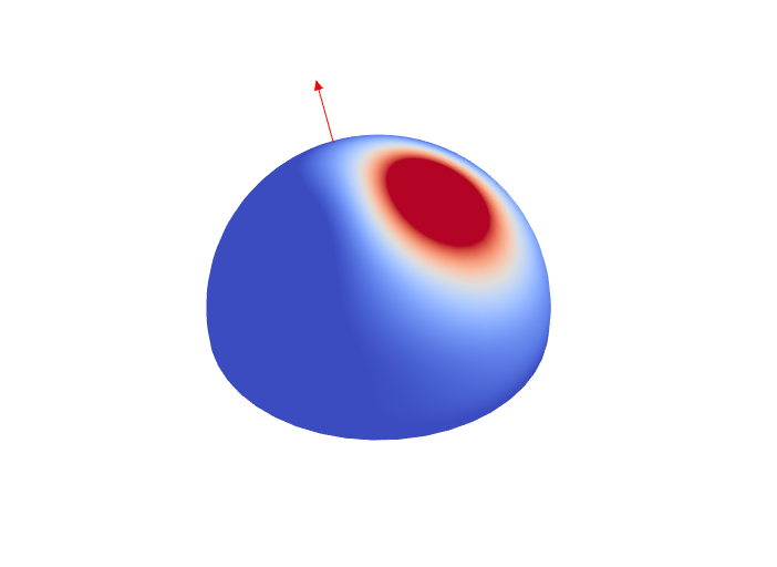
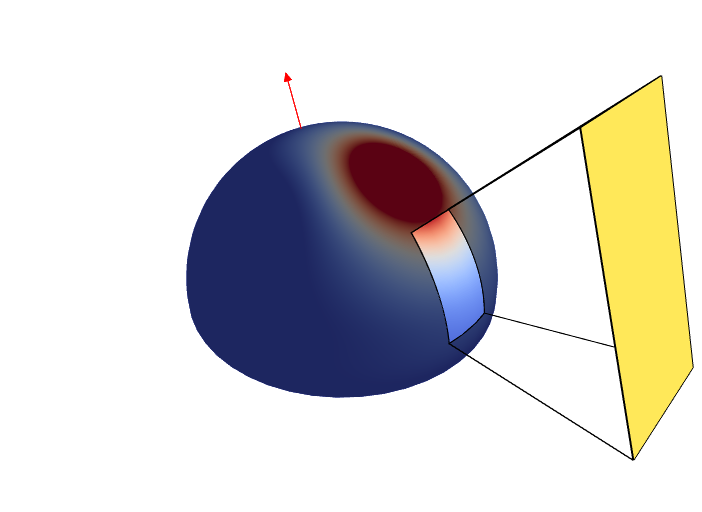
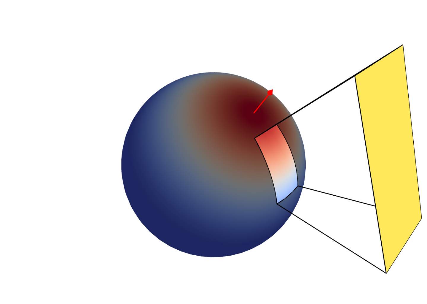
Outline of Our Method

$$ \int_\mathcal{P} f(\boldsymbol\omega) \mbox{d}\boldsymbol\omega $$

$$ \sum f_{l,m} \int_\mathcal{P} y_{l}^{m}(\boldsymbol\omega) \mbox{d}\boldsymbol\omega $$

$$ \sum c_{k,i} \int_\mathcal{P} \langle \boldsymbol\omega \cdot \boldsymbol\omega_i \rangle^{k} \mbox{d}\boldsymbol\omega $$

lobe sharing

Now, here is how our method works. To compute the integral of a spherical function over a spherical polygon, *click*

we use its spherical harmonics decomposition illustrated here. There, we need to compute the integral of each basis element over the spherical polygon. *click*

But instead of trying to solve this task, we show how to convert any spherical harmonics expansion into a set of rotated power cosines for which we can compute the exact integral. So, we remap our problem of integration to a problem of conversion which is much simpler to solve. *click*

To ensure that our method is efficient, we share the same axis for different axial moments and share the computation of the integral.

Insight: An Intermediate Step

Rotated Zonal Harmonics [Nowrouzezahrai et al. 2012]

Decomposing Rotated Zonal Harmonics

That's All Folks!

                            
/* Compute the integral of the SH decomposition with
 * `f` coefficients over a spherical polygon `poly`.
 */
function ComputeIntegral(flm, poly) {
    
    // Generate a set of vectors
    basis = SharedDirections();

    
    // Compute the conversion matrices
    //   `A` converts SH to Zonals
    //   `P` converts Zonals to Axials
    A  = ZonalWeights(basis);
    P  = AxialWeights(basis);
    AP = A*P;

    
    // Convert the Axial expansion
    cpw = flm.transpose() * AP;

    
    // Return the integral using Arvo's method
    m = AxialMoments(poly, basis);
    return cpw.dot(m);
}

$$ \mathbf{f}^T \mathbf{y} = \sum_{l,m} \mathcal{\color{green}{f_{l,m}}} \left[ \int_{\mathcal{\color{darksalmon}{P}}} y_{l,m}(\omega) \right] $$

$$ \mathbf{c}^T = \mathbf{f}^T \times AP $$

$$ \mathbf{f}^T \mathbf{y} = \underbrace{\mathbf{c}^T}_{\mathbf{f}^T \times AP} \times \mathbf{m} $$

That is pretty much it for out method. Now we can put everything toghether in the following algorithm. *click*

Our goal is to compute the integral of all the Spherical Harmonics functions over a polygon P. Then to compute the weighted sum of those integral to get the integral we are interested in. *click*

First, we need to precompute a set of axis for the zonal decomposition. *click*

Then, we compute the conversion matrix `A` that converts spherical harmonics coefficients into rotated zonal harmonics coefficients. We also compute the conversion matrix `P` that converts zonal harmonics into rotated cosine powers. *click*

Then, we compute the cosine powers coefficients by multiplying the conversion matrices to the Spherical Harmonics coefficients. Note that for efficiency, we should always precompute those coefficient ahead. Here we detail all those aspects in place for clarity. *click*

Last, we compute the integral by doing the dot product between the rotated cosine power coefficents and the axial moments computed using Arvo's method. *click*

That's All Folks! (How Really?)

Redudant computation in Arvo's method

We improve performance by
- sharing axial moment directions
- sharing Arvo's recursive evaluation

Details are in the paper

However, the devil is in the details and a naive implementation of this algorithm could lead to poor performance. *click*

When converting a rotated zonal harmonics in a rotated cosine power, we did not pay attention to the fact that redudant computation will occur in Arvo's integration method. *click* For example, *click* if we were to compute the integral of the two rotated power cosine hihglihgted here in green independently, due to the recursive form the Arvo's algorithm, we would recompute the same arc integrals twice.

The idea to ensure good performance is to couple the main axis of the rotated zonal harmonics across bands to share computation in Arvo's method. *click* In the zonal decomposition showed on the right, *click* the same axis is shared by different order of rotated zonals harmonics. *click* During the computation of Arvo's method, the recursive evaluation of the line integral will be shared across all orders distributing the cost of the integration. *click*

For more details regarding the implementation, please refer to our paper and supplemental code. *click*

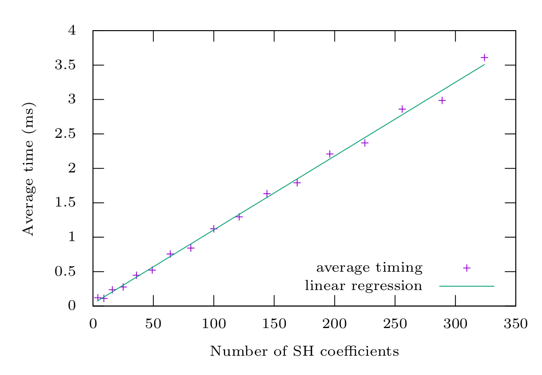
Algorithmic Complexity

Linear w.r.t. number of SH coefficients

Applications

real-time rendering importance sampling
hierarchichal warping control variate
adding shadows

We applied our integration method to different case scenarios. *click*

Thanks to its efficiency, we performed a GPU implementation of our method for the real-time rendering of area-lights. There, efficiency is a requirement. *click*

Importance sampling of Spherical Harmonics decomposition can be acheived using Hierarchial Warping. This method relies on the decomposition's integral on spherical quads. We applied our method there as well. *click*

Finally, we demonstrated our integration method in an offline rendering scenario. There, we looked at how to incorporate shadows and how to correct for the approximation caused by the Spherical Harmonics decomposition. To that purpose, we applied control variate. *click*

I will only detail this last method. To know more about the other two, please refer to our paper.

Surface and Volume Shading

[Arvo 1995]

Surface area light

Surface portal light

Volume area light

Volume portal light

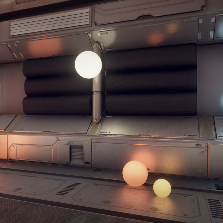
Surface Shading: Area Light

Surface area light

$$ \color{green}{\rho(\boldsymbol{\omega}_i, \cdot}) \simeq \mathbf{f} = \mathbf{y}_i^T, \mbox{M} \quad \mbox{with} \, \, \mathbf{y}_i = y_{l,m}(\boldsymbol{\omega}_i) $$ [Westin et al. 1992]

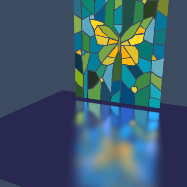
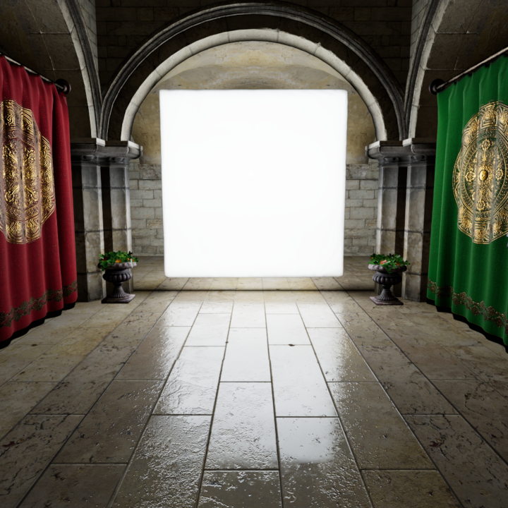
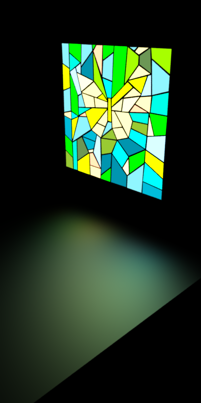
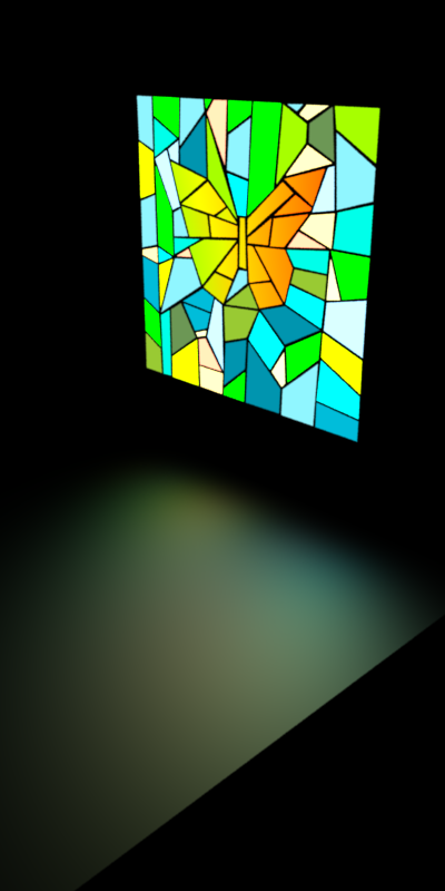
Surface Shading: Portal Light

Surface portal light

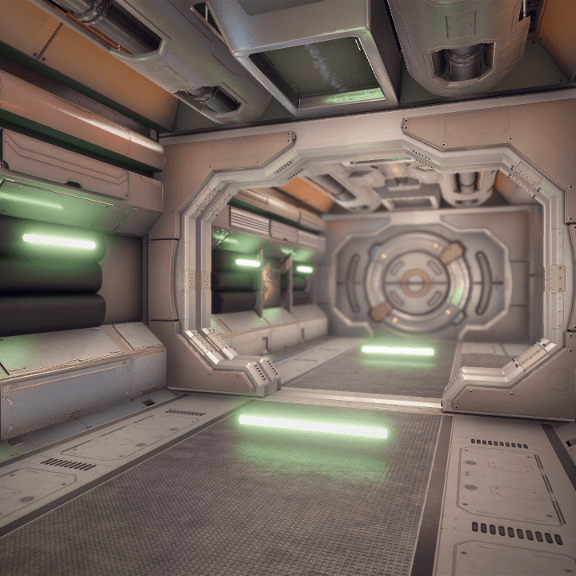
Volume Shading: Area Light

Volume area light

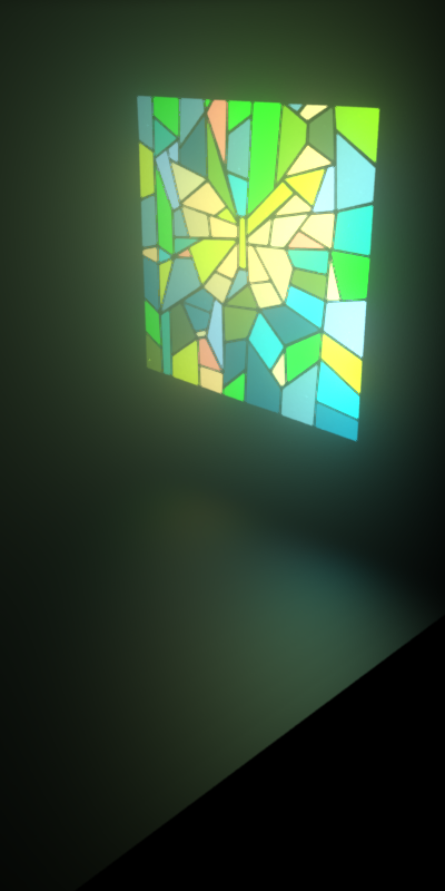
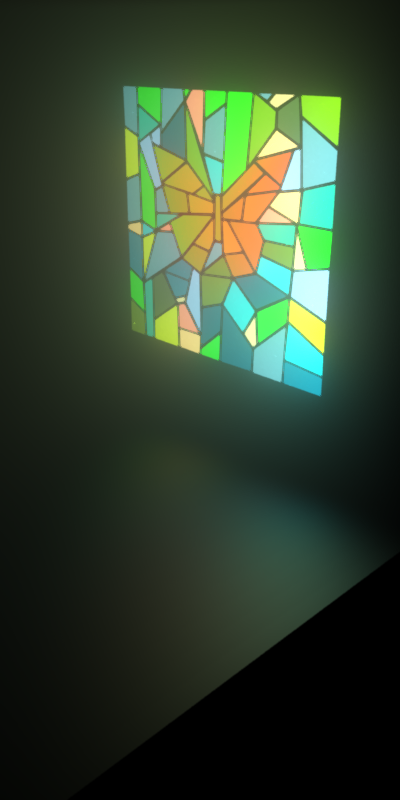
Volume Shading: Portal Light

Volume portal light

Application: Real-Time Rendering

Application: Control Variates

Our real-time demo lacks shadows

Analytical solutions have bias
- they do not account for shadows
- they approximate the true BRDF
Combine Closed-Form and Monte-Carlo results
$$ I = \color{green}{\int_{\mathcal{P}} y\left(\boldsymbol\omega\right) \mbox{d}\boldsymbol\omega} \, - \, \color{blue}{\sum_{k} \left[ y\left(\boldsymbol\omega_k\right) - f\left(\color{blue}{\boldsymbol\omega_k}\right) \right]} $$
Visual 'Side effect'
- No noise in unshadowed regions
- Ensure unbiasness w.r.t. $f(\boldsymbol{\omega})$

Unfortunately, the analytical integration fails to account for parts of the rendering equation. *click* The first issue is the inability of the SH integral to account for shadowing as you can see on this image from our real-time demo. It is possible to bake the shadows into the SH decomposition but this is prohibitive and requires many coefficients. The second source of error is that the SH decomposition is an approximation of the true signal to integrate. *click*

We used control variate to overcome those bias. The idea here is to correct the closed-form integral with a Monte-Carlo estimator. *click*

There, the closed-form solution is corrected by a Monte-Carlo estimator that compute the difference between the spherical harmonics integral and the exact integrand noted f here. This later integrand contains the shadow and/or the correct BRDF. *click*

The target effet is to get a resulting radiance that is noise free in region where the SH decomposition has no bias. That is in unshadowed region we will get a large reduction in variance. Also, we can build an unbiased estimator when this criteria is critical.

Application: Control Variates

Dragon scene

Application: Control Variates

Fog scene

Application: Control Variates

San Miguel scene

Summary

We integrate Spherical Harmonics
- over spherical polygons
- with a closed-form expression
- that is efficient (linear cost)
We apply this new tool
- to surface and volume shading
- to polygonal portal lights
- to importance sampling

Thank you for your attention


paper	code

available at belcour.github.io/blog