SIGGRAPH 2016 Course: Part 1

This course note is the first part of the 2016 SIGGRAPH course on Frequency Analysis of Light Transport. Additional material such as slides and source code are available in the main page. Note: most of the diagrams and figure are interactive (but not all of them). Please feel unashamed to click on them!

Introduction

The idea of Frequency Analysis of Light Transport as sketched by Durand and colleagues [2005] is that many tools used in rendering are better understood using a signal processing approach. Not only can we explain phenomena such as soft shadows and glossy reflections, but we can also improve existing algorithms. For example, Frequency Analysis enables to improve denoising and adaptive sampling algorithms, density estimation or antialiasing.

Signal processing uses an alternative representation of a signal which: its Fourier transform. A Fourier transform describes a signal in terms of amplitude with respect to frequency instead of the traditional view (we call the primal) that describes a signal in terms of amplitude with respect to coordinates.

Mathematically, the Fourier transform of a signal \(f(\mathbf{x})\) where \(\mathbf{x} = [x_1, \cdots, x_N] \in \mathbb{R}^N\) is:

Here, variable \(\mathbf{\Omega} = [\Omega_1, \cdots, \Omega_N] \in \mathbb{R}^N\) describes the frequency domain coordinates.

The Fourier transform has many interesting properties that we will uncover as we need them. For more information about it, you can go to its wikipedia page. The next step is to specify how the Fourier transform is applied in rendering.

Fourier Transform of Radiance

We need to perform our frequency analysis from first principles governing the rendering of images. In physically based rendering, this is provided by the Rendering Equation [Kajiya 1986] that describe the conservation of radiance energy at surface boundaries:

Here \(\mathbf{y}\) is the directly visible point from \(\mathbf{x}\) in direction \(\boldsymbol{\omega}^\prime\). The surface material is represented by the bidirectional reflectance distribution function \(\rho(\boldsymbol{\omega}, \boldsymbol{\omega}^\prime)\). The emission from surfaces is noted \(L_e\). And \((\cdot, \cdot)^{+}\) is the clamped dot product to positive values.

However, this expression is not simple to perform frequency analysis due to its recursive nature and to the direction \(\boldsymbol{\omega}\) (The usual Fourier transform is defined over a planar domain). We will see in the following how this recursion can be used to build frequency estimate.

Bandwidth

The bandwidth of a signal is its Fourier transform’s extent. Mathematically, the bandwidth is the minimum support of the signal’s Fourier transform. It provides information on the necessary sampling pattern to either reconstruct it or to integrate it. Intuitively, it gives the maximum amount of relative variation a signal has. This is enough to predict the maximum distance between samples for perfect sampling. This is however assuming that the bandwidth is finite (or distance between samples would be zero).

Covariance Tracing is a method to evaluate the bandwidth of the local radiance around a given light path. Knowing the bandwidth of the radiance enable a lot of applications (see [1-3]). This document present the idea of covariance tracing and frequency analysis in a progressive way.

For simplicity, we will illustrate the different concepts using 2D light transport.

Local Fourier Transform

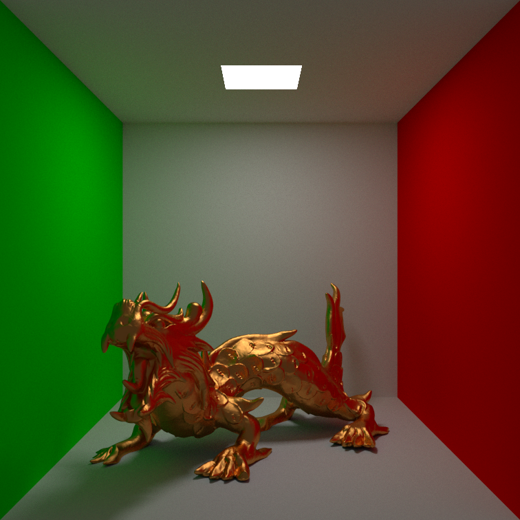
However, using the Fourier transform defined previously, it would be hard to develop a fine analysis. For example, if we look for the bandwidth of the rendering image of the dragon above, we will find that the bandwidth if infinite due to the hard edges. Instead, we will use a local frequency analysis defined with respect to a central point.

Using a local windowed Fourier transform, we can perform a finer analysis and differentiate between low frequency regions (green inset) and high frequency regions (red inset). It requires a different formulation of the Fourier transform. You can move the local window in the frame.

Mathematically, we will incorporate this notion of windowing into the definition of the Fourier transform:

where \(W_l(\mathbf{x}_0 - \mathbf{x})\) is a windowing function of size \(l\) around point \(\mathbf{x}_0\).

In the following, to ease notation, we will note the local Fourier transform of the radiance as \(\hat{l}(\Omega_x, \Omega_u) = \mathcal{F}_l[L](\Omega_x, \Omega_u)\).

What is covariance?

In the following, we will talk about covariance referring to the covariance of the Fourier transform of the radiance function. The covariance is a matrix describing the orientation and spread of a signal. Covariance gives us an indication on the bandwidth of the signal and enable to work with signals having infinite bandwidth.

Since we are interested by 2D light transport, we will use a 2D matrix. The complete formulation of covariance tracing involves a 5D matrix (2D in space, 2D in angles and 1D in time).

 cov = { sxx, sxy;
         syx, syy };

where sxx and syy are the variance (or squared standard deviation) of the signal along the x (and respectively y) axis of our domain. sxy = syx is the correlation of the signal with respect to axis x and y. A covariance matrix is symmetric and this property can be used for efficient implementation.

Ray Local Space

In order to describe the radiance for small perturbation of a given ray, we need a parametrization of this local space. We will use the tangential space defined by the ray. This space can be defined using a two plane parametrization.

Mathematically, we express positions and directions as perturbations of the main position (resp. direction) along the tangent plane of the ray:

Now that we have this parametrization, we can express the radiance in that space: \(L(\mathbf{x}_0 + \delta \mathbf{x}, \boldsymbol{\omega}_0 + \delta \mathbf{u} )\). But remember that we are interested by its Fourier transform. While local radiance is parametrized in 2D by the couple \((\delta{x},\delta{y})\), it is parametrized by the couple \((\Omega_x,\Omega_u)\) in the Fourier domain.

The next step is to express radiance transport equations in this space and to convert them using the Fourier transform.

Radiance Operators in Local Space

Expressing the Rendering Equation or the Radiative Transfer Equation in local coordinates is not possible since they rely on global coordinates. Instead, we look at solutions of those equations for simple cases (operators) that correspond to transport evaluated during path tracing. We will need to describe several transport operators such as travel in free space, reflection, refraction, etc..

Remember that we are not interested in the resulting radiance, but to its Fourier transform. What we really want is how an operator affects the Fourier spectrum. Fortunately, under a first order assumption (equivalent to paraxial optics), we can formulate analytically how operators modify it. Furthermore, we will have the same analytical formulation for the covariance matrix.

The travel operator

The travel operator is the simplest of all. It describes the local radiance given that we now the local radiance from a previous position along the ray. Using the tangent plane formulation described earlier, we can update the local position of a ray after a travel of length d. Only the spatial component of the ray will be updated since the ray’s direction remains fixed.

This operator shears the local radiance by the amount of traveled distance. The equivalent operator on the covariance matrix is also a shear which parameter is the traveled distance in meters. However, in the Fourier domain, the shear transfers spatial content to the angular domain. This is the opposite behaviour for radiance. It can be understood in the limit case where the travel distance is infinite. There, locally around the central direction of the ray, only radiance along the same direction remains. Thus the angular content is locally a dirac (a single direction) and the spatial content is locally a constant (same radiance for neighboring positions).

Mathematically, the local radiance after \(d\) meters is expressed as:

Since we are interested by a first order approximation of the radiance, we can approximate \(\tan(\delta u) \simeq \delta u\). After this approximation, the Fourier transform of the local radiance can be expressed analytically as:

A Matlab implementation of the operator is the following:

  // Express the covariance after a travel of 'd' meters
  function travel(d) {
     op = { 1, d;
            0, 1};
     cov = op' * cov * op;
  }

The visibility operator

Since we are studying local radiance, we need to account for the fact that part light might be occluded or that part of the light will not interact with an object. We account for those two effects by reducing the local window used for our frequency analysis until there is no more near-hit or near-miss rays. Applying a window to a signal means that we will convolve its Fourier spectrum by the window Fourier spectrum:

This translate into a convolution in the Fourier domain:

We usually assumes that occluders are planar. In such case, we can perform the windowing on the spatial component only. If an occluder has non negligible depth, then we can slice it along its depth and apply multiple times the occlusion operator. In terms of covariance, this boils down to summing the covariance matrices.

  function occlusion(w) {
     occ = {w, 0;
            0, 0};
     cov = cov + occ;
  }

The projection operator

The projection operator enables to express the local radiance and the covariance in the tangent plane of objects. This is necessary to express the reflection or refraction of light on a planar surface. When the surface is non-planar, the curvature operator is applied after this operator.

Intuitively, this operator scales the spatial frequency content to match the new frame. Imagine that the incoming radiance is unidirectional and which a structured pattern. If you account for the difference of travel with respect to the tangent plane, some ray will have to travel further than other. Thus the distance with respect to the central position will scale with respect to the angular difference between the incident local plane and the tangent plane and the structured pattern will be dilated. Dilatation of space reduces frequency in the Fourier domain, this is why we have a cosine scaling in the operator.

Mathematically, the projected local radiance on the plane with normal \(\mathbf{n}\) is expressed as:

This translate into the Fourier domain as:

A Matlab implementation of the operator is the following:

  function project(cos) {
     op = {cos, 0;
             0, 1};
     cov = op' * cov * op;
  }

The BRDF operator

The BRDF operator describes how the roughness reduces the bandwidth of the reflected local radiance. This is well known that the BRDF can be thought as being a blurring filter (think of pre-filtered envmaps).

This operator describes the integral product of the incoming local radiance with the BRDF. For an isotropic BRDF model, it is possible to express the outgoing radiance using a convolutive form:

This translate into a product in the Fourier domain:

The BRDF operator is not easy to define using the covariance matrix. Intuitively, we want to express the covariance of the product of two signals using their respective covariance matrices. If we have no knowledge of the type of signals we are multiplying, then this product is undefined. However, in the case of Gaussians spectra the product is defined as the inverse of the sum of the inverse covariance matrices.

  function BRDF(B) {
     cov = inverse(inverse(cov) + B);
  }

where B describe the angular blur of the BRDF. It is defined using the inverse of the absolute value of the BRDF’s Hessian in the tangent plane of the reflected ray. For a Phong BRDF with exponent e with a reflected ray in the pure mirror direction, the matrix is defined as:

 B = { 0, 0;
       0, 4*pi^2/e};

The curvature operator

So far we have expressed how to trace the covariance of local radiance when light is reflected by planar objects. To incorporate the local variation of the object’s surface into covariance tracing, we will enable to project the local radiance from the tangent plane to a first order approximation of the surface using its curvature.

Mathematically, the first order approximation of the projected local radiance on a sphere of curvature \(k\) is expressed as:

The Fourier transform of the local radiance can be expressed analytically as:

In terms of covariance, the operator is expressed similarly to the travel operator:

  function curvature(k) {
     op = { 1, k;
            0, 1};
     cov = op' * cov * op;
  }

In the next section, we will see how to pratically use the knowledge of the Fourer spectrum extents.