Part II: Frequency Operators
< previous partOverview
- Introduction
- Frequency Operators
- Travel & Occlusion
- Reflection & Refraction
- Scattering & Absorption
- Applications
- Adaptive sampling & denoising
- Upsampling
- Density estimation
- Antialiasing
- Conclusion
Fourier Transform of Radiance
$$
\mathcal{F}[L](\Omega) = \int_{\mathbf{z} \in \mathbb{R}^N} L(\mathbf{z}) e^{i 2 \pi \, \mathbf{\Omega}^T \delta\mathbf{z}}, \; \mbox{where} \; \mathbf{z} = [\mathbf{x}, \mathbf{\omega}]
$$
- This cannot in practice: global definition
- Need to treat the whole scene at once
- Actually not well-defined (discontinuous domain)
Local Fourier Transform of Radiance
- local FT requires a window: $ W_l $:
$$ \mathcal{F}_l[L](\Omega) = \int_{\mathbf{z} \in \mathbb{R}^N} L(\mathbf{z}) \ \color{red}{ W_l(\mathbf{z}) }\ e^{i 2 \pi \, \mathbf{\Omega}^T \mathbf{z}}, \; \mbox{where} \; \mathbf{z} = [\mathbf{x}, \mathbf{\omega}] $$
- Interesting properties:
- Makes the Fourier Transform well defined
- The window increase the min frequency
Local Fourier Transform of Radiance
- We aren't looking at point-wise radiance anymore
- Local radiance around a main ray
- Requires a parametrization
$$L(\mathbf{x}, \boldsymbol{\omega})$$
$$L(\mathbf{x} + \delta\mathbf{x}, \boldsymbol{\omega}+ \delta\boldsymbol{\omega})$$
Local Fourier Transform of Radiance
- We aren't looking at point-wise radiance anymore
- Local radiance around a main ray
- Requires a parametrization
Local Fourier Transform of Radiance
- We aren't looking at point-wise radiance anymore
- Local radiance around a main ray
- Requires a parametrization
- Constraint: analytical forms
- First order analysis (only consider linear properties)
- In practice we represent the spectrum
Local Rendering Equation
Rendering Operators
- Implementation example
- Manipulation of the covariance matrix
- Using Matlab's' syntax
Cov = {sxx, sxu;
       sxu, suu};
First Step Operators: Surface Shading
 Durand et al. 2005
Travel Operator
Travel Operator
- Travel is a shear in local space
% Travel of 'd' meters
Tr  = [1, d; 0, 1]
Cov = Tr' * Cov * Tr
Durand et al. 2005
Egan et al. 2011
Visibility Operator
Visibility Operator
- Add frequencies in the spatial domain
- Has infinite bandwidth!
% Visibility operation
Occ = [o, 0; 0, 0]
Cov = Cov + Occ
Visibility in Practice
- Same as ajusting the local window
- Compute the largest unoccluded disk along the ray
- We will treat near misses the same way as near hit
- Requires a special treatment/data-structure
- Voxel grid
- Distance field
- Shadow map discontinuities
Shading Operators
- Shading requires to decompose
- Final travel to the surface (projection)
- Material (Textures / BSDF)
- Elements we won't cover
- Foreshortenning scale the spatial componnent
- Texture increase the spatial componnent
Durand et al. 2005
Curvature Operator
Curvature Operator
- Curvature shears angular frequencies
% Projection to a curved object of radius 'k'
Cv  = [1, 0; k, 1]
Cov = Cv' * Cov * Cv
Durand et al. 2005
Reflection Operator
BRDF roughness: 0 0.05
Reflection Operator
- The BRDF cuts the angular frequency
- Acts as a low-pass filter
- Cutof depends on the BRDF lobe
% BRDF with cut at 'b'
B   = [0, 0; 0, b]
Cov = inverse(inverse(Cov) + B)
BRDF is not All!
 Belcour 2012
Refraction Operator
Refractive index: 1 3
Refraction Operator
- Snell laws scale the angular component
- Critical angle as a windowing (increase freq. near TIR)
- Rough refraction as low pass filter on top
% Snell interface with e=n1/n2
Tf = [1, 0; 0, e*i.z/t.z]
Cov = Tf' * Cov * Tf
Adding Defocus!
Soler et al. 2009
Lens Operator
- A compound of already seen operators!
- Curvature and transmission in the lens
- Travel to the sensor
Lens Operator
- For thin lenses, it simplifies to
- Curvature plus Travel operators
% Lens with focal length f and distance to sensor d
C   = [1, f; 0, 1]
Tr  = [1, 0; d, 1]
L   = C * Tr
Cov = L' * Cov * L
Adding Motion-Blur
Adding Another Dimension for Motion-Blur
- A new dimension: time.
Cov = {sxx, sxu, sxt;
       sxu, suu, sut;
       sxt, sut, stt};
- Easy formulation: coordinate change.
Motion Operator
Egan et al. 2009
Belcour et al. 2013
Motion Operator
- Motion is a shear in space/angle/time
- Our local Fourier Transform window follows the motion
- Need to apply the operator twice (before and after interaction)
% Occlusion with moving object of speed 'vx'
M   = [1, 0, vx; 0, 1, 0; 0, 0, 1]
O   = [o, 0, 0; 0, 0, 0; 0, 0, 0]
Cov = M * (M' * Cov * M + O) * M'
Adding Volumes
Belcour et al. 2014
Participating Media Operators
- Using a different rendering equation:
- Radiative Transfert Equation [Ishimaru 1978]
- Still defined on the radiance $ L(\mathbf{x}, \omega) $
Absorption Operator
- Same operator as occlusion
- However not an infinite bandwidth
Scattering Operator
- Same operator as BRDF
- Analytical forms for the Henyey-Greenstein phase function
- Need to be aligned with the outgoing ray
- Add a scale in the spatial domain
- Same as projection with no curvature
Summary: Frequency Operators

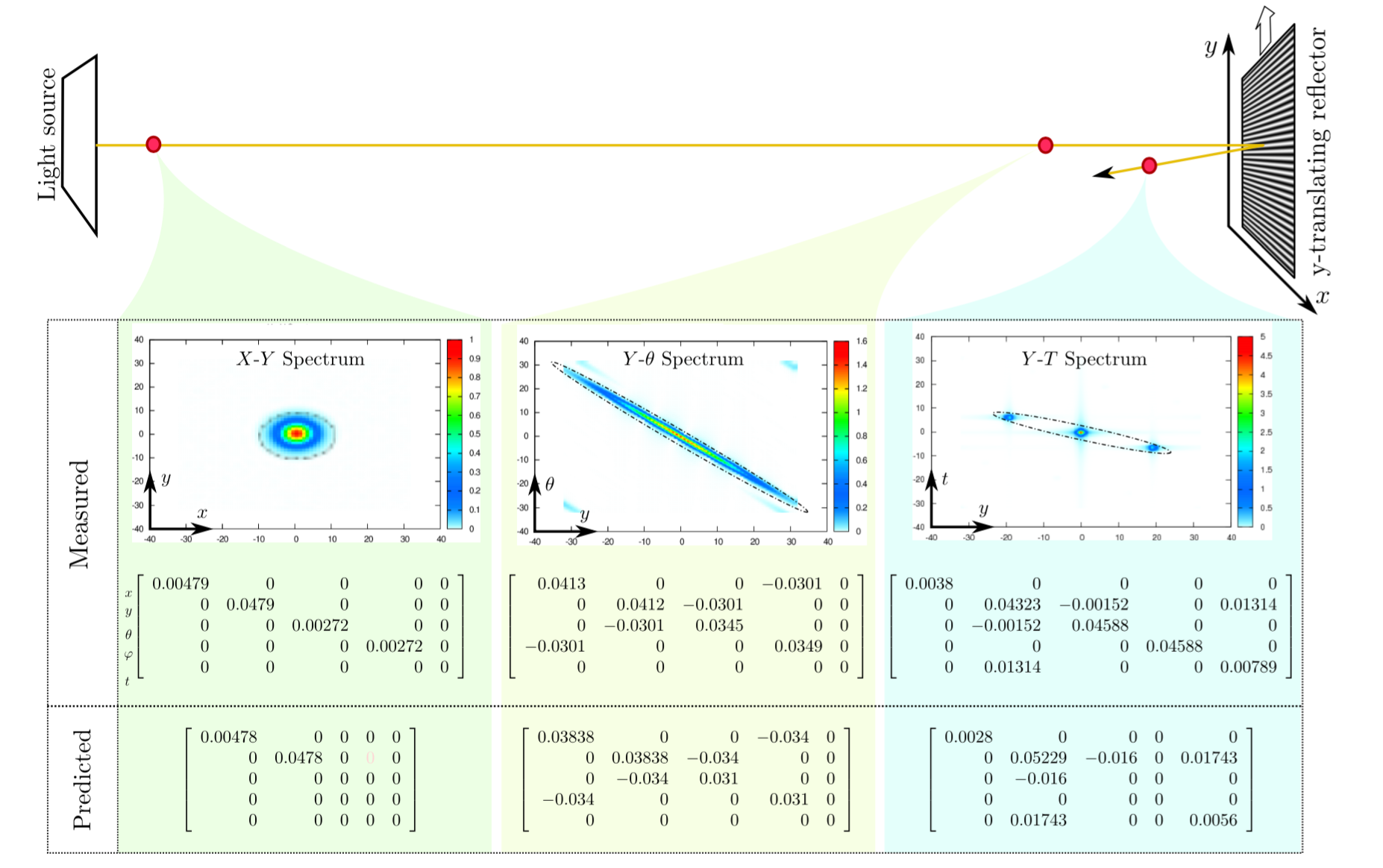
Validation
Summary: A Unified Theory
Break: Questions?
> next part