Part III - Applications
< previous partOverview
- Introduction
- Frequency Operators
- Travel & Occlusion
- Reflection & Refraction
- Scattering & Absorption
- Applications
- Adaptive sampling & denoising
- Upsampling
- Density estimation
- Antialiasing
- Conclusion
Overview
- Introduction
- Frequency Operators
- Travel & Occlusion
- Reflection & Refraction
- Scattering & Absorption
- Applications
- Adaptive sampling & denoising
- Upsampling
- Density estimation
- Antialiasing
- Conclusion
Working with Operators
'Deferred' Frequency Analysis
- Static analysis: using closed forms
- Compatible with you favorite math toolbox
- Last example with Mathematica

'Deferred' Frequency Analysis
- Need a pre-pass to compute the spectrum
- During G-buffer creation for interactive
- During a sampling pre-pass for offline
'Online' Frequency Analysis
- When closed forms are not possible
- Multiple scattering dominant
- Multiple scenarios but same code (reflexion and refraction)
- Inline frequency analysis in raytracing
- See source code on github
Spectrum RayTrace(Ray r){

   // Check intersection
   hit = Intersect(scene, r);
   if(! hit) return Black;

   // Interaction with material
   Ray new_r = SampleBRDF(hit);
   return RayTrace(new_r);
}
>
Spectrum RayTrace(Ray r, Covariance c){

   // Check intersection
   hit = Intersect(scene, r);
   if(! hit) return Black;

   // Evaluate covariance at the surface
   c.Travel(hit);
   c.Projection(hit);

   // Interaction with material
   Ray new_r = SampleBRDF(hit);

   // Compute reflected covariance
   c.Reflection(hit);
   c.InverseProjection(hit);

   return RayTrace(new_r, c);
}
Application to Adaptive Sampling & Reconstruction
Adaptive Sampling and Reconstruction
- Direct application of Nyquist:
- Adapt the sampling rate w/r $ B_W $
- Reconstruct using a kernel (usualy Gaussian)
- Share samples across pixels
- Avoid over-sampling when not needed
Adaptive Sampling and Reconstruction
- However a specific context:
- Reconstruct in pixel space
- Integrate in lens/light/time space
Adaptive Sampling and Reconstruction
- Algorithm:
- Compute bandwidth per pixel
- Sample XYUVT space
- Integrate in UVT space & reconstruct in XY space
 Soler et al. 2009
Adaptive Sampling and Reconstruction
- Example of lens integration
- Operators: Reflection + Travel + Occlusion + Lens
- Adapt the sampling of the lens and in screen space
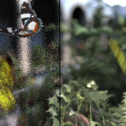
Results
Alternative Methods
- Gradient adaptive sampling
- Heuristic adaptive sampling

Application to Upsampling
Bagher et al. 2013
Upsampling
- Dual of reconstruction
- Instead of gather samples for a pixel, splat them
- Equivalent to shade bigger pixels
Bagher et al. 2013
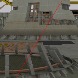
Upsampling
Alternative Methods
- Shading bigger pixels
- Global-Illumination upsampling [Nichols et al. 2009]
- Coarse Pixel Shading [Vaidyanathan et al. 2014]
- Splatting more samples
- Off-line resampling [Lehtinen et al. 2011, Lehtinen et al. 2012]
Application to Photon Mapping
Belcour and Soler 2011
Adaptive Density Estimation
Density Estimation
- Initial radius has a big impact
- At the core of some modern techniques:
Adaptive Density Estimation
- Mathematical insight:
- Density estimation blurs the target result
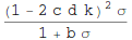
- Theoretically: $ \mbox{bias} \propto \mbox{Laplacian} \times \mbox{radius}^2 $
Adaptive Density Estimation
- How to Estimate Laplacian?
- Covariance in Fourier = Hessian!
- Covariance from photons is averaged for each kernel
- Works as well in volumes
- Adapt kernels for the Photon Beams method [Jarosz et al. 2011]
- Covariance must be stored in a 3D grid
Results
Results
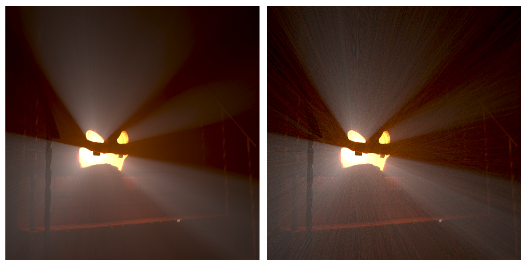
9.7M beams, 25min render10M beams, 25min render
Alternative Methods
- Progressive Hessian estimation


Application to Antialiasing
 Belcour et al. 2015
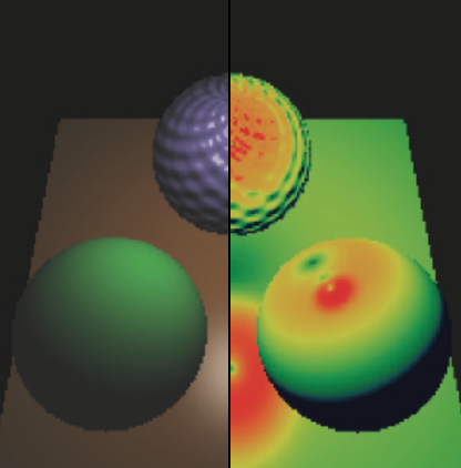
Antialiasing Surface Appearance
- Idea: bound the reflectance frequencies
- Adapt variation to screen resolution
 |
 |
|---|---|
| Ground truth | Nearest evaluation |
Image from Mitsuba [Wenzel Jakob]
Antialiasing Surface Appearance
Antialiasing Surface Appearance
Limitation of Decoupling & Pixel Footprint
- Break with bidirectional path-tracing (BDPT, VCM)
- Light variations must be accounted
- Assume the view and light directions are constant
- Using a 'binary'' footprint
- Doesn't account for the pixel filter
- Limited to single scattering
Antialiasing Surface Appearance
- Pixel filter is a kernel applied on the surface!
Frequency Analysis Perspective
- This kernel is a low-pass filter on the SV-BRDF:
Antialiasing and Global Illumination
- The kernel can account for multiple bounces:
- How can we estimate the kernel in that case?
Covariance Antialiasing
Comparison to Ground Truth Kernel
Kernel after one bounce
Bidirectional Antialiasing
Bidirectional Antialiasing
Bidirectional Antialiasing
$$ \Sigma_e \; + \; \Sigma_l \; = \; \Sigma $$
Alternative Methods
- Predict filtering footprint
- Ray differentials [Igehy 1999]
- Path differentials [Suykens and Willems 2001]
- Antialiasing distant lighting
- Filtered Importance Sampling [Krivanek and Colbert 2009]
- Rough transmission [De Rousiers et al. 2012]


Practical Considerations
Light Sources
- Need Fourier spectrum for each light type
- Analytical forms for point, spot and area
- For envmaps, we need to numerically compute its FFT
Textures
- Albedo texture
- FFT Required for 'online' analysis
- For single scattering it is better to decouple from shading
- Roughness texture
- Correlates spatial and angular frequencies
- In practice we only consider spatial
- Mip-level for different windows
BRDFs/BSDFs
- Need analytical forms in practice
- Not always the case (microfacets)
- Use conversion to Phong (approximate is good enough)
- Get the Hessian is an alternative [Belcour et al. 2014]
- Measured data (e.g. MERL)
- Store a 2D texture of FFT slices [Bagher et al. 2012]
Break: Questions?
> next part